Merge Sort And It's Early History

Illustrated guides to become better engineers

Few people know about merge sort, I stand by the statement. Even fewer people know about its history. Merge sort is vaguely stated to be invented by Von Neumann. Yes, but when exactly? In what context? I assure you, the current Wikipedia entry is of no help! This post is dedicated to explaining merge sort along with its history.

To explain the original merge sort, we’ll take a ride through computer architecture and early assembly language. The merge sort program is not just any program, it’s a core piece of computing as it was designed as a test for both programming languages and computer architecture.

Knuth dives for the meshing manuscripts

The original program for merge sort is one of the earliest computer programs. Donald Knuth took the pain to look for the first manuscript and events surrounding merge sort. He published the finding under the title: “Von Neumann’s First Computer Program“. Please read it to better understand this post. Entries listing Knuth’s algo book as a reference for Neumann’s authorship are very weird.

Knuth found the original manuscripts with Herman Goldstine, someone with whom Neumann collaborated. Only the merging process called meshing is described in this document. The actual algorithm is described in the 3-part series called “Planning and Coding of Problems for an Electronic Computing Instrument“, co-authored by Goldstine.

Background

This was at a time when computer architecture was still in development. Around the 1930s-1940s, electronic calculators were being used. Some people felt the need for high-speed computing using the same principles as calculators. Analog machines like the Differential Analyzer were being used at the time. Eckert, a young electrical engineer drew up a plan for an electrical machine at the Moore School. After this, the US government helped fund research at the institution in this direction. This culminated in the ENIAC machine with Eckert as chief engineer. The EDVAC machine was an improvement over the ENIAC among others by switching the parallel circuitry approach to a serial one. Neumann became a consultant for the project.

Architecture and programming background of the original program

In order to understand Neumann’s first program, it’s important to understand the context behind it, or else the code does not make much sense.

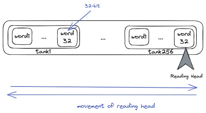
Neumann proposed a serial computer with 3 32-bit registers and 8132 32-bit words of auxiliary memory. The 3 registers were called: i (input), j (input), and o (output, referred to by Knuth as A). The EDVAC memory was planned to be divided into 256 sections called tanks of 32 words each, operating in a cyclic fashion. The head restarts at the beginning after reading the last word.

This can also be represented conceptually as this

This cyclic fashion of reading was concretely implemented in head-per-track disks.

The first bit of a word denoted whether the word was a number or an instruction. A typical number was represented in reverse order with the sign bit at the end.

Decimal coded integers were also allowed in the format 0000 a1…a4b1…b4 … g1…g4

Instructions were stored in the format of 1 a0…a4 b0…b2 0000000000 y0…y4 x0…x7

a denoted an operation code
b denoted a variant
y0 + 2 y1 + 4 y2+ 8 y3 + 16 y4 denoted a word position within a tank

x0 + 2 x1 + 4 x2 + … +128 x7 denoted a tank number.

These are the codes for a

This means that if we have registers in this state

And the program reads

which is the instruction for AD, it will load values from I and J, add them then insert the result in A

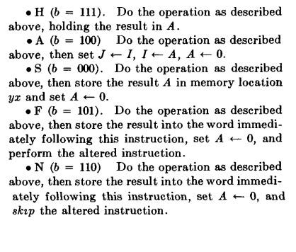
This is what the b part means

Since the b part offers more flexibility,

ADS yx, where (yx is the word-tank location omitted in the diagram) represented by this

means, as seen above, set location yx to I+J and clear A to 0.

Besides adding and substracting, the machine could also execute

Further codes like a = 01010, 01011, 01100, 01101, 01110, 01111 were reserved for input and output operations (not yet specified) and stopping the machine.

I and J registers contained only numbers. When the LOD operations specified a memory address containing an instruction, only the yx part of that instruction was to be loaded into I; the other bits were cleared. When storing into memory by using variants S, F, and N, only the least significant 13 bits of the number in A were to be stored in the yx part, if the memory location contained an instruction word.

Execution was sequential unless a JMP statement was found. If the word is a number, it is taken as if a LOD instruction is done using that number.

So, using this system, we have instructions to modify and refer to memory. This is not a great design but it was a great start for both architecture and programming.

Improved EDVAC code

He also designed a second version and added 32 “short tanks“ whose capacity was one word, replacing I and J registers.

It also had 2048 additional words in 64 long tanks. He imagined this memory sufficient to tackle all problems. He also improved the instructions, some of them are shown below.

let C(s) denote the contents of short tank number s

Timing

The time to read one bit was called a bit-time, estimated at 1 µsec.

So, a word-time would be 32 µsec.

In the original one, most instructions took one word-time. But multiplication, radix conversion etc took 33 word-time. Memory access would require an additional 1024 µsec.

In the improved one, TRA instruction (long-tank switching) took 2 word-time.

About the original program

The program was written in this format, very maths-like:

Knuth explained it in terms of assembly.

It was a test case concerning the capabilities of programs to control process flows. In our time, control structures and data are coded in one and same program. It was not so at the time.

Sorting was chosen as a topic to compare computer speed “time taken“ against IBM’s specialized sorting machines.

The original program did not include sorting. It had only the merging part explained.

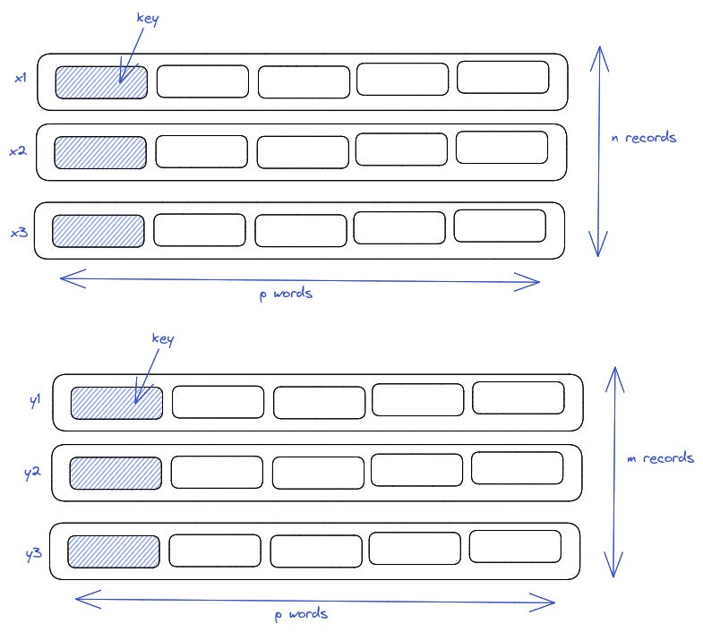
It wanted to merge n and m records each having p words in one merged sequence.

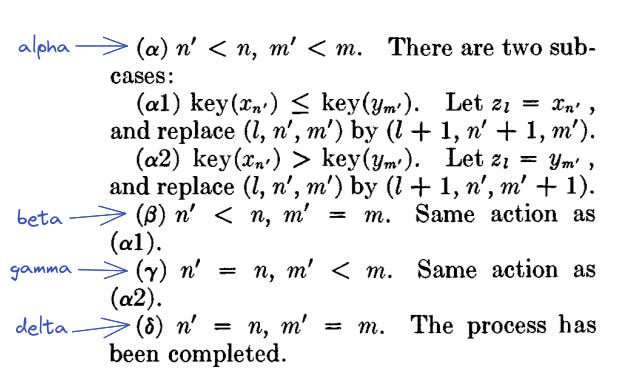
He referred to the merged sequence as z.

He had 4 cases for the control flow

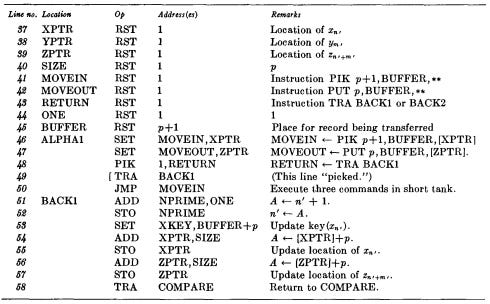
The below program is written in actual assembly language by Knuth. It has RST for an imaginary Reserve Short Tank, EQU for equivalence, CON for integer constant, * denotes the current location, and ** denotes an address filled in dynamically.

We see that the first 15 lines set addresses, referred to later on in the code.

Remarks are not to be ignored. They contain descriptions of what’s going on.

This shows the complete program. e is an imaginary starting point for the addresses. This post is enough for you to follow the program.

There is a refined implementation mentioned in “Planing And Coding of Problems For An Electronic Computing Instrument” which discusses sorting. But the whole thing is so ugly an explanation using custom symbols etc that it deserves a post of it’s own.

Typical implementation

A traditional approach to merge sort involves these steps:

• Knowing how to merge two sorted arrays

• Recurse and merge when array length is equal to one

• Find an in-place variant

This program has nothing to do with Von Neumann.

Merging two sorted arrays

Merging two sorted arrays involves moving the pointer in each one after selecting the element to be added to the sorted list. Both pointers start at the beginning.

We start with the first array, then the second.

We continue doing so until all elements are in the list.

The remaining elements are added in after the initial comparison.

Recurse and merge when array length is equal to one

The typical explanation is this

The coding can be something as elegant as this.

Instead of copying lists, we can modify the actual list as Python supports referencing. This converts it to an in-place implementation.

Conclusion

Merge sort and derivatives like Timsort are undoubtedly fascinating. But, Neumann’s take on things is even more entertaining to dive in.